- K-armed Bandit Problem
- Confidence based exploration
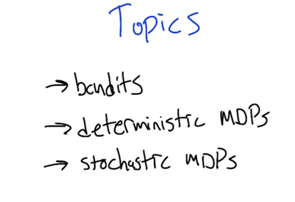
- Metrics for Bandits
- Find Best Implies Few Mistakes
- Few Mistakes Implies Do Well
- Do Well Implies Find Best
- Hoeffding
- Combining Arm Info
- How Many Samples?
- Exploring Deterministic MDPs
- Rmax Analysis
- General Rmax
- What Have We Learned?
This week
- Watch Exploration.
- The readings were Fong (1995) and Li, Littman, Walsh (2008).
| Type | state transition | Stochastic | solution |
|---|---|---|---|
| Bandits | ✘ | ✔ | hoeffding bound to do stochastic decision making |
| Deterministic MDPs: | ✔ | ✘ | Rmax to do sequential decision making |
| Stochastic MDPs | ✔ | ✔ | both hoeffding bound and Rmax |
K-armed Bandit Problem
- Each slot has a probability to get certain payoff or no payoff
- Payoff or the associated probabilities are unknown.
- what’s the best thing to do? Exploration.
Confidence based exploration
!Quiz 1: K-Armed Bandits, given the observed data, which arm gives the ightest expected payoff and which arm are most comfident](/assets/images/计算机科学/118382-6578df35f8c00073.png)
- arm d gives 1 pay off in the smallest number of try
- arm g gives most reliable output since it’s been pulled the most and gives a good payoff.
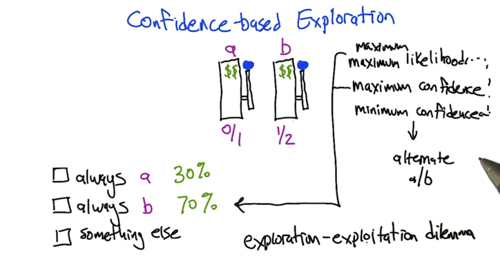
- Maximum Likelihood: ① Given current info, figure out the best expected action based on best likelihood -> ② act, and get new info -> repeat ① ② will always choose b
- Maximum Confidence: ① Given current info, figure out the best expected action based on best confidence -> ② act, and get new info -> repeat ① ② will also choose b only
- Minimum Confidence: ① Given current info, figure out the best expected action based on smallest confidence -> ② act, and get new info -> repeat ① ② will also choose to alternating between a and b. But it will not favor the better arm.
- Exploration-exploitation dilemma: combine maximum maximum likelihood and minimum confidence. The latter allows to try different actions and the former allows us to choose the best reward.
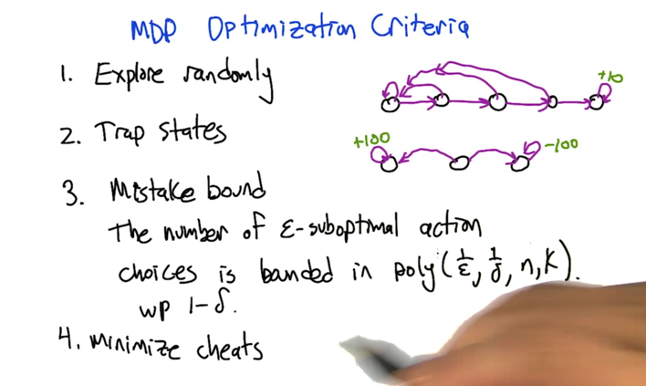
Metrics for Bandits
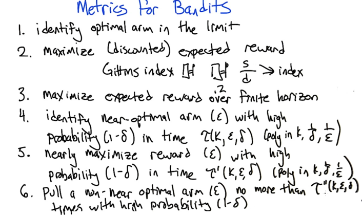
- identify optimal arm in the limit: exploration
- maximize (discounted) expected rewards: exploration + exploitation, but computationaly expensive
- Gittins index: a real scalar value associated to the state of a stochastic process with a reward function and a probability of termination.
- Gittins index works well with Bandits, should not generalize to other RL.
- Maximize expected reward in finite horizon - similar to value iteration
- Identify near-optimal arms (ε) with high probabilities ( 1- δ) in time τ(k, ε, δ) (polynomial in k, 1/ε, 1/δ) - The “get there” goal is to find near optimal arms. similar to PAC learning: probably approximately correct.
- Nearly Maximize reward (ε) with high probabilities ( 1- δ) in time τ’(k, ε, δ) (polynomial in k, 1/ε, 1/δ): the “how to get there” goal is to accumulate as much more rewards as possible in finite time τ’.
- Pull a non-near optimal arm (ε) no more than τ’‘(k, ε, δ) times with high probabilities ( 1- δ): The “control error” goal is to minimize mistakes.
Find Best Implies Few Mistakes
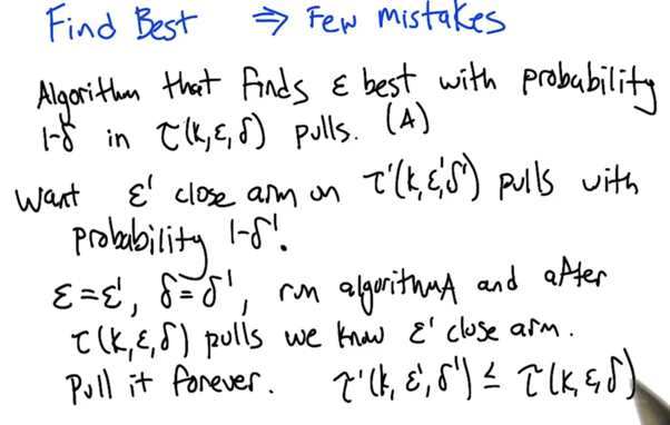
- τ’ is the total number of mistakes when we find ε’ close arm
- τ’ is bounded to τ.
Few Mistakes Implies Do Well
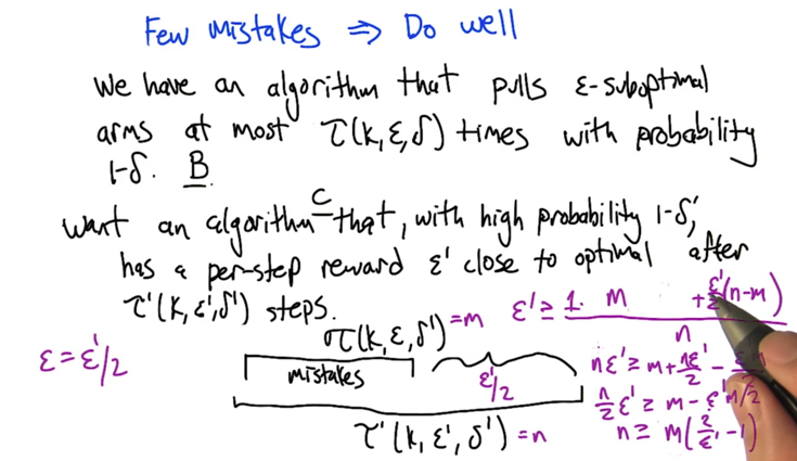
- is it true that the smaller the m is, the smaller the n is? not always.
- but it is true that the smaller the m is, the small the n could be.
- “Do well” means algorithm C can lead to ε’ close to optimal arm where ε’ < ε.
Do Well Implies Find Best
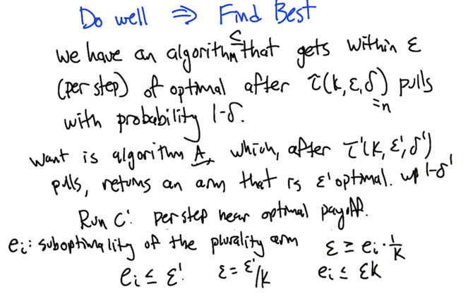
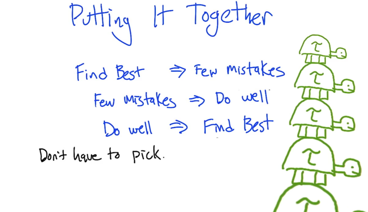
- Given algorithm of one goal, we can derive algorithms to reach the other two.
- So there is no need to pick one.
- need to know that the three goals are not always solvable (so you might have to pick one?).
Hoeffding
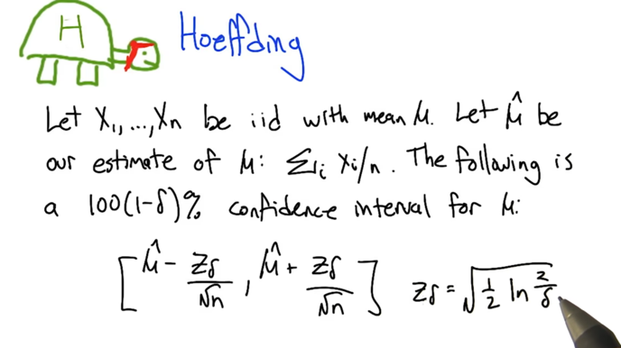
- 0 <= δ <=1. The more confident we are the smaller the δ -> the larger the Zδ -> the larger the confidence interval
- the larger the n is, the smaller the confidence interval
Combining Arm Info
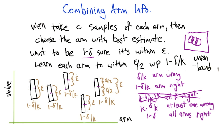
- the length of the bar, ε, is the confidence interval of μk.
How Many Samples?
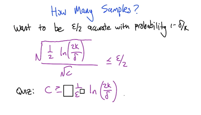
- C depends more on ε and less on δ (δ is in ln)
- PAC-style bounds for bandits.
Exploring Deterministic MDPs
- in MDP, we can only choose action but not state
- we can treat action selection as bandit problem (e.g. k action is a k arm bandit).
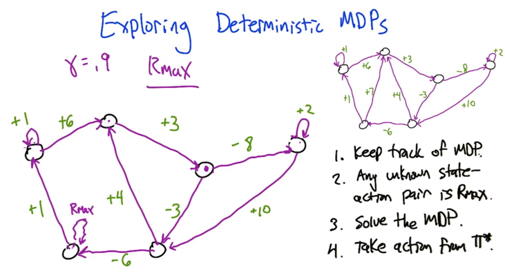
- Rmax: assume any state we have not full explored (unknown state-action pair) has a self-loop of reward Rmax.
- This way, the learner is encouraged to explore the whole MDP.
Rmax Analysis
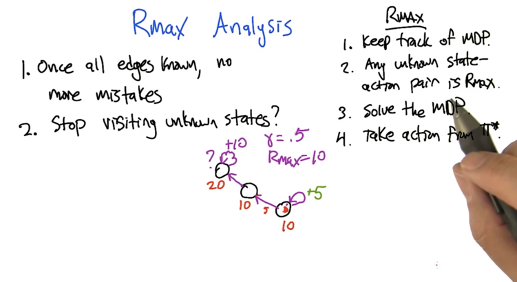
- the example: even with Rmax, there is a possibility that the learning stops visiting unknown states
- discount factor is important to determine if the agent is going to explore unknown edge.
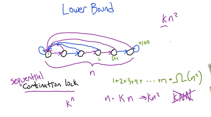
- We have a upper bound saying the algorithm can solve the problem with n2k steps
- now we are proving that no other algorithms can take less than n2k steps
- The sequential combination lock has n states, in each state the learner can take k actions.
- at i th state, one action can send the learner to next state (i + 1), all other actions will take the learner to state 0, to get back to state i, the learner has to take at least i steps (the worst case deterministic MDP).
- In the worst case, it might take kn2 steps to solve a deterministic MDP before stopping make mistakes.
General Rmax
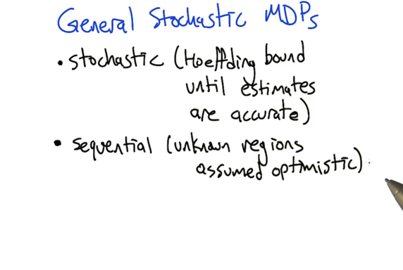
For Stochastic properties, applying hoeffding bound. For sequential deterministic MDP, Rmax can solve the problem. Now applying both, we can solve the stochastic MDP.
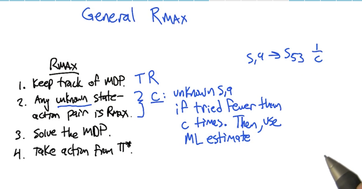
- For Rmax algorithm, define Unknown s, a pair as: if tried fewer than C times. Then use maximum likelihood estimate.
- the C part is hoeffding bound.
Some key ideas for this to work: Simulation Lemma and Explore-or-Exploit Lemma
Simulation Lemma
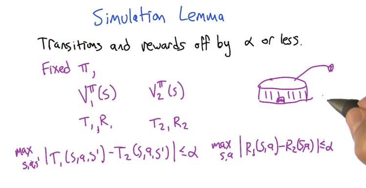
- if we get an estimated MDP that is close to real MDP, then the optimizing the reward based on the estimate will be very close to the optimal policies for the real MDP.
- α is the difference between estimated and real MDP.
- α could be different if transition possibility and reward are not in the same scale, but we can alway rescale things to that α is between 0 and 1.
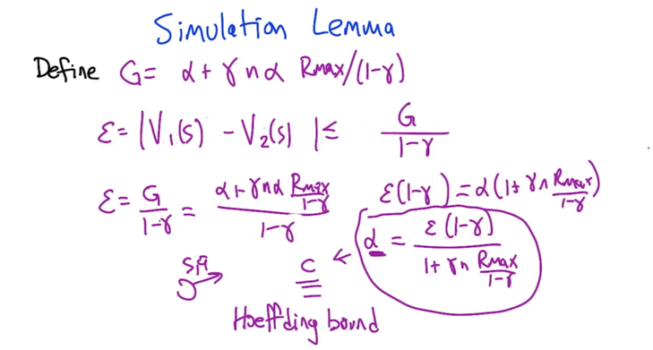
- α is related to ε
- α is used to determine C
- using Hoeffding bound and union bound to find a big enough C which can estimate an MDP which is close enough to real MDP.
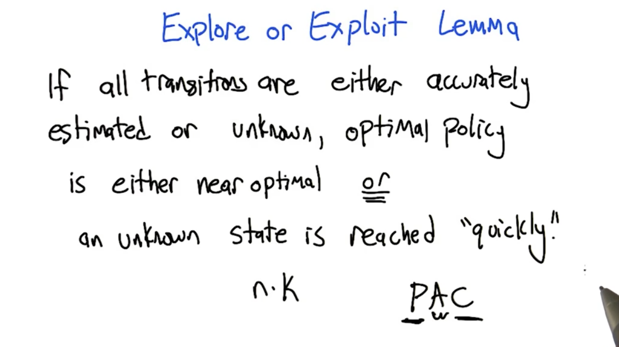
Explore-or-Exploit Lemma
What Have We Learned?
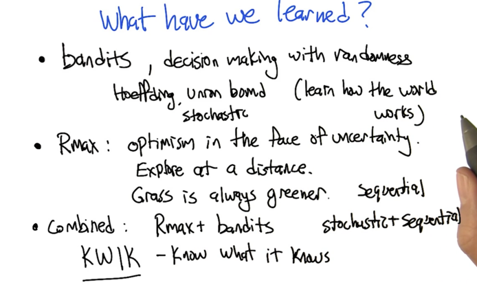
- Hoeffding bound and Union bound let us know how certain we are about the environment
- Rmax makes sure we “visited” things enough to get accurate estimates
2015-10-06 初稿 up-to quiz 1
2015-10-07 updated to Exploring Deterministic MDPs
2015-12-04 reviewed and revised